

Microsoft Excel 2010 Conditional Formatting feature enables you to format a range of values so that the values outside certain limits, are automatically formatted.
Choose Home Tab » Style group » Conditional Formatting dropdown.
Various Conditional Formatting Options
Highlight Cells Rules − It opens a continuation menu with various options for defining the formatting rules that highlight the cells in the cell selection that contain certain values, text, or dates, or that have values greater or less than a particular value, or that fall within a certain ranges of values.
Suppose you want to find cell with Amount 0 and Mark them as red.Choose Range of cell » Home Tab » Conditional Formatting DropDown » Highlight Cell Rules » Equal To.
 After Clicking ok, the cells with value zero are marked as red.
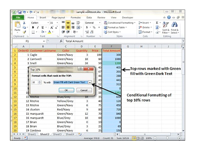
 Top/Bottom Rules − It opens a continuation menu with various options for defining the formatting rules that highlight the top and bottom values, percentages, and above and below average values in the cell selection.
Suppose you want to highlight the top 10% rows you can do this with these Top/Bottom rules.
 Data Bars − It opens a palette with different colour data bars that you can apply to the cell selection to indicate their values relative to each other by clicking the data bar thumbnail.
With this conditional Formatting data Bars will appear in each cell.
 Colour Scales − It opens a palette with different three- and two-coloured scales that you can apply to the cell selection to indicate their values relative to each other by clicking the colour scale thumbnail.
See the below screenshot with Colour Scales, conditional formatting applied.
 Icon Sets − It opens a palette with different sets of icons that you can apply to the cell selection to indicate their values relative to each other by clicking the icon set.
See the below screenshot with Icon Sets conditional formatting applied.
 New Rule − It opens the New Formatting Rule dialog box, where you define a custom conditional formatting rule to apply to the cell selection.
Clear Rules − It opens a continuation menu, where you can remove the conditional formatting rules for the cell selection by clicking the Selected Cells option, for the entire worksheet by clicking the Entire Sheet option, or for just the current data table by clicking the This Table option.
Manage Rules − It opens the Conditional Formatting Rules Manager dialog box, where you edit and delete particular rules as well as adjust their rule precedence by moving them up or down in the Rules list box.
Choose Home Tab » Style group » Conditional Formatting dropdown.
Various Conditional Formatting Options
Highlight Cells Rules − It opens a continuation menu with various options for defining the formatting rules that highlight the cells in the cell selection that contain certain values, text, or dates, or that have values greater or less than a particular value, or that fall within a certain ranges of values.
Suppose you want to find cell with Amount 0 and Mark them as red.Choose Range of cell » Home Tab » Conditional Formatting DropDown » Highlight Cell Rules » Equal To.


Suppose you want to highlight the top 10% rows you can do this with these Top/Bottom rules.

With this conditional Formatting data Bars will appear in each cell.

See the below screenshot with Colour Scales, conditional formatting applied.

See the below screenshot with Icon Sets conditional formatting applied.

Clear Rules − It opens a continuation menu, where you can remove the conditional formatting rules for the cell selection by clicking the Selected Cells option, for the entire worksheet by clicking the Entire Sheet option, or for just the current data table by clicking the This Table option.
Manage Rules − It opens the Conditional Formatting Rules Manager dialog box, where you edit and delete particular rules as well as adjust their rule precedence by moving them up or down in the Rules list box.


0 Comments